Key Terms — Query Performance
Query Profile
Snowsight's visual execution plan for a completed query — shows operator tree, timing, pruning stats, and spilling information.
Micro-Partition Pruning
Snowflake's automatic optimisation that skips micro-partitions whose metadata (min/max) indicates they cannot match the query's WHERE clause.
Spilling
When query intermediate data exceeds warehouse memory and overflows to local SSD, then to remote cloud storage — a key performance warning sign.
Result Cache
A 24-hour Cloud Services cache that returns identical query results instantly with zero warehouse credits.
EXPLAIN
SQL command that shows the logical execution plan without actually running the query — no credits consumed.
Scale Up
Increasing warehouse size to provide more memory/compute per query — fixes spilling.
Scale Out
Adding multi-cluster capacity to handle more concurrent queries — fixes queueing.
Query Lifecycle
Every SQL statement in Snowflake follows the same execution path through three layers:
Query Execution Flow
Flow diagram: 1) User submits SQL. 2) Cloud Services Layer parses, optimises, and creates execution plan. 3) Virtual Warehouse executes the plan against micro-partitions in cloud storage. 4) Results returned via Cloud Services Layer. Each step labelled with what happens: parse/compile, optimise/prune metadata, distribute to compute nodes, scan/join/aggregate, return result set.
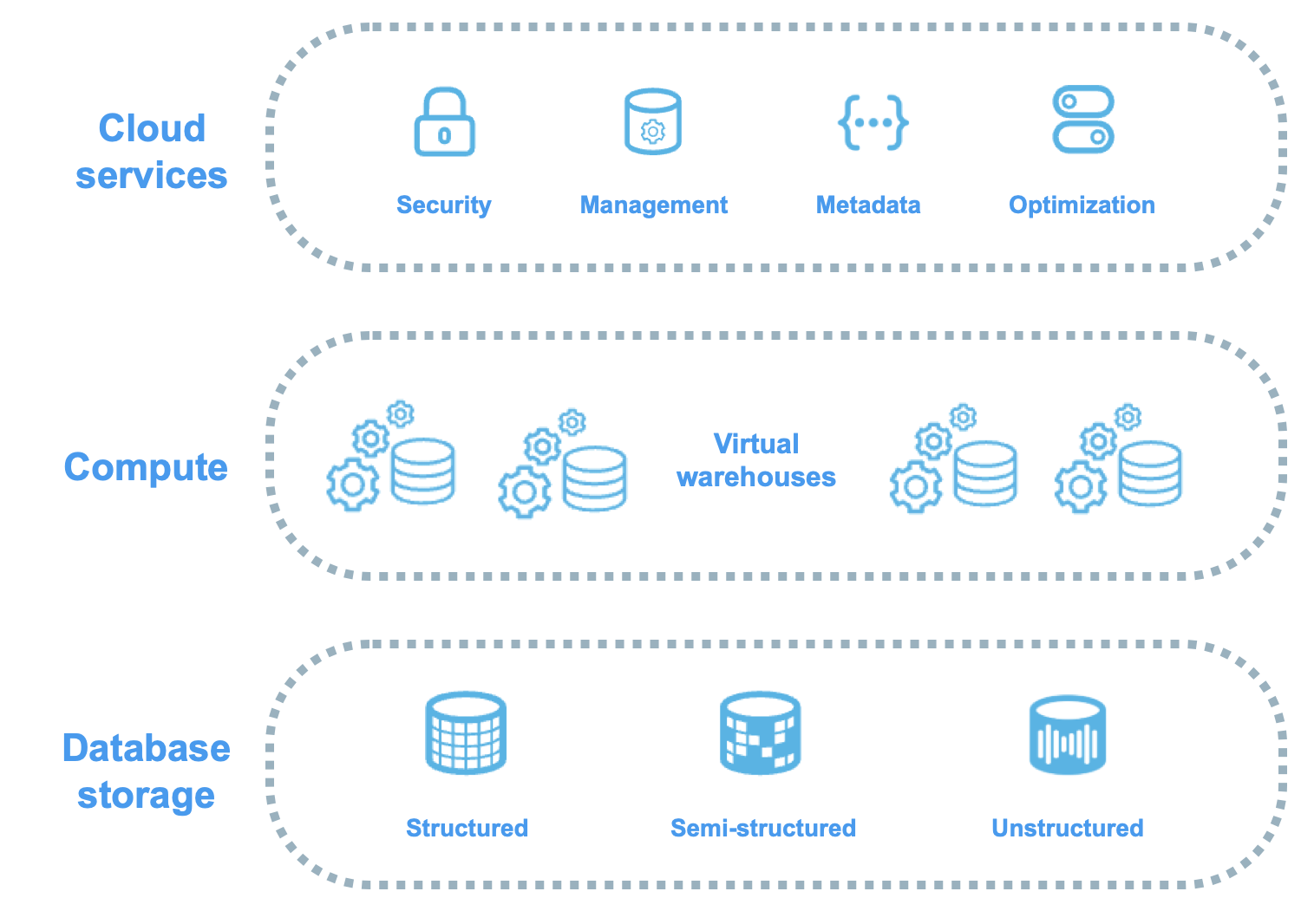
- Cloud Services — parses SQL, resolves objects, checks privileges, generates optimised execution plan, determines which micro-partitions to scan
- Virtual Warehouse — executes the plan: scans micro-partitions, applies filters, performs joins, aggregations, and sorts
- Cloud Services — returns results to client, caches result for potential reuse
Unlike traditional databases, Snowflake has no indexes to create, no statistics to update, and no VACUUM to run. The query optimiser uses micro-partition metadata (min/max, NDV, null counts) automatically. Your main levers for performance are: warehouse sizing, clustering keys, and writing efficient SQL.
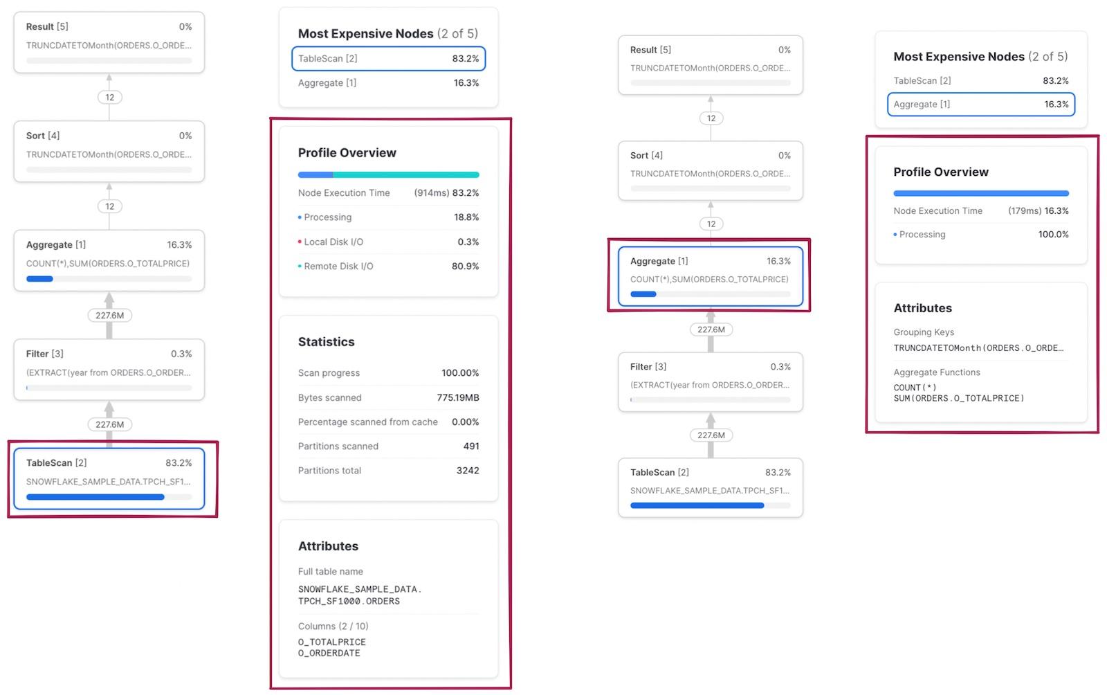
The Query Profile
The Query Profile in Snowsight is your most important diagnostic tool. It shows the actual execution plan as a tree of operator nodes.
Query Profile Operator Tree
Tree diagram of a typical Query Profile: Result node at top, below it an Aggregate node, feeding into a Join node with two branches — left branch shows TableScan on ORDERS with Filter, right branch shows TableScan on CUSTOMERS. Each node shows percentage of total time, rows processed, bytes scanned. The Join node consumes 45% of time. The TableScan shows partitions scanned 120 of 5000 total, indicating good pruning.
Key Operator Nodes
| Node | Purpose |
|---|---|
| TableScan | Reads micro-partitions from storage — shows pruning stats |
| Filter | Applies WHERE clause predicates |
| Join | Combines data from multiple tables (hash join, merge join) |
| Aggregate | GROUP BY, COUNT, SUM operations |
| Sort | ORDER BY and merge join preparation |
| Exchange | Redistributes data between compute nodes — often the most expensive |
What to Look For
- Partitions scanned vs total — Is pruning effective?
- Bytes spilled to local/remote storage — Is the warehouse too small?
- Percentage bars — Which operators consume the most time?
- Exploding joins — Does a join produce far more rows than its inputs?
1-- Get the last query's ID2SELECT LAST_QUERY_ID();34-- Retrieve operator stats for any query5SELECT *6FROM TABLE(GET_QUERY_OPERATOR_STATS(LAST_QUERY_ID()));Micro-Partition Pruning
Pruning is Snowflake’s primary query optimisation. Every micro-partition stores column-level metadata (min/max values). When your WHERE clause specifies a range or equality predicate, Snowflake compares the filter against each partition’s metadata and skips partitions that cannot contain matching rows.
Micro-Partition Pruning in Action
Eight micro-partitions labelled MP1-MP8 with date ranges. A WHERE clause for dates in February prunes 6 partitions (greyed out) and scans only 2 partitions (highlighted green). Shows: Partitions scanned 2 of 8 total — 75% pruning efficiency.
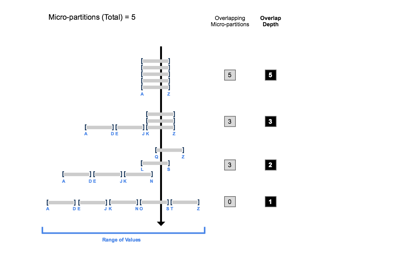
Applying a function to a column in WHERE disables pruning on that column. WHERE YEAR(order_date) = 2024 prevents Snowflake from using min/max metadata. Rewrite as WHERE order_date >= '2024-01-01' AND order_date < '2025-01-01' to preserve pruning.
1-- Run a filtered query and check Query Profile for partition stats2SELECT order_id, customer_id, order_date, total_amount3FROM sales.orders4WHERE order_date BETWEEN '2024-06-01' AND '2024-06-30'5AND region = 'EMEA';67-- In Query Profile, click TableScan node:8-- Partitions scanned: 150 / Partitions total: 12,0009-- = 98.75% of partitions prunedSpilling to Disk
When a query’s intermediate data exceeds warehouse memory, Snowflake spills data through a hierarchy:
Spilling Hierarchy
Three-tier pyramid: Top (green) = Memory/RAM (fastest, all processing ideally here). Middle (amber) = Local SSD (slower, data spills when memory exceeded). Bottom (red) = Remote Cloud Storage S3/Blob/GCS (slowest, severe performance degradation). Arrows point downward labelled Overflow.
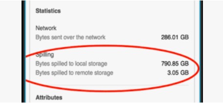
The primary fix for spilling is to increase warehouse size (e.g., Medium to Large). Each size doubles memory and compute. If spilling persists, also optimise the query: reduce data volume with better filters, avoid SELECT *, or break into smaller steps with temporary tables.
1SELECT query_id, query_text, warehouse_name, warehouse_size,2 execution_time / 1000 AS exec_seconds,3 bytes_spilled_to_local_storage,4 bytes_spilled_to_remote_storage5FROM snowflake.account_usage.query_history6WHERE bytes_spilled_to_remote_storage > 07ORDER BY bytes_spilled_to_remote_storage DESC8LIMIT 20;Query History
INFORMATION_SCHEMA vs ACCOUNT_USAGE Query History
The exam tests the difference: INFORMATION_SCHEMA = 14 days, real-time, database-scoped. ACCOUNT_USAGE = 365 days, 45-minute latency, full account.
EXPLAIN Command
1-- Logical plan without execution (zero credits)2EXPLAIN USING TABULAR3SELECT c.name, SUM(o.total) AS total_spend4FROM customers c5JOIN orders o ON c.id = o.customer_id6WHERE o.order_date >= '2024-01-01'7GROUP BY c.name8ORDER BY total_spend DESC;910-- EXPLAIN shows operators and expected rows11-- Query Profile shows ACTUAL execution after completionWarehouse Sizing Strategy
Warehouse Sizing Decision Process
Identify the Problem
Check Query Profile for spilling, poor pruning, or queue times. Examine top 10 slowest queries via ACCOUNT_USAGE.
Spilling? Scale Up
Increase warehouse size (Medium to Large, Large to X-Large). Each step doubles memory and compute.
ALTER WAREHOUSE analytics_wh SET WAREHOUSE_SIZE = 'X-LARGE';Queueing? Scale Out
Enable multi-cluster warehouses (Enterprise+). Adds clusters for concurrent queries.
ALTER WAREHOUSE analytics_wh SET
  MAX_CLUSTER_COUNT = 3
SCALING_POLICY = 'STANDARD';Over-provisioned? Scale Down
If queries finish in seconds with no spilling, use a smaller warehouse to save credits.
ALTER WAREHOUSE dashboard_wh SET WAREHOUSE_SIZE = 'X-SMALL';Scale Up vs Scale Out
Scale Up vs Scale Out
Common Anti-Patterns
- SELECT * on large tables — reads all columns, Snowflake is columnar — specify only needed columns
- Functions on WHERE columns — disables pruning: WHERE YEAR(date) = 2024
- Unnecessary DISTINCT — forces expensive sort/aggregate
- Cartesian joins — missing join conditions
- Wrong data types — VARCHAR compared to NUMBER forces implicit casting
- Overly complex CTEs — deeply nested CTEs can confuse the optimiser
Cheat Sheet
Query Performance Quick Reference
Query Profile
AccessPruningSpillingWarehouse Sizing
SpillingQueueingResult CacheQuery History
INFO_SCHEMAACCOUNT_USAGEPractice Quiz
A Sort operator is spilling 50 GB to remote storage. What is the MOST appropriate fix?
A user runs the same SELECT twice in 10 minutes. Data unchanged. Warehouse is suspended. What happens on the second run?
A query filters WHERE YEAR(created_at) = 2024. Only 200 of 10,000 partitions are pruned. What is the best fix?
Flashcards
What are the two spilling locations and which is worse?
First: local SSD (attached to warehouse nodes). Second: remote cloud storage (S3/Blob/GCS). Remote spilling is much slower and indicates the warehouse should be scaled up immediately.
What three conditions must be met for the result cache to fire?
1) Exact same SQL text. 2) Underlying data unchanged since caching. 3) Same role and context (database, schema). Cache lasts 24 hours. No warehouse needed — served from Cloud Services.
INFORMATION_SCHEMA vs ACCOUNT_USAGE: retention and latency?
INFORMATION_SCHEMA: 14 days, real-time, current database. ACCOUNT_USAGE: 365 days, up to 45-minute latency, full account scope.
How does EXPLAIN differ from Query Profile?
EXPLAIN shows the logical plan BEFORE execution — zero credits. Query Profile shows ACTUAL execution AFTER completion — real timing, data volumes, and spilling.
When should you scale up vs scale out?
Scale UP: individual queries are slow or spilling (more memory per query). Scale OUT (multi-cluster): many concurrent queries queueing (more clusters for concurrency).
Resources
Next Steps
Reinforce what you just read
Study the All flashcards with spaced repetition to lock it in.