Data Storage & Clustering
Snowflake’s storage layer is fundamentally different from traditional databases. Understanding how micro-partitions work, how data is physically organised on disk, and how clustering influences query performance is essential knowledge for the COF-C02 exam.
This module covers the Database Objects & Storage domain of the COF-C02 exam. Expect 2–4 questions on micro-partition internals, clustering key configuration, and storage billing across table types. Pay particular attention to when clustering keys are — and are not — recommended.
1. Micro-Partitions: The Foundation of Snowflake Storage
Every table in Snowflake is divided into micro-partitions — the fundamental unit of Snowflake’s physical storage. Unlike traditional databases that require you to manually define partitions, Snowflake creates and sizes micro-partitions automatically with no intervention required.
Micro-Partition Architecture
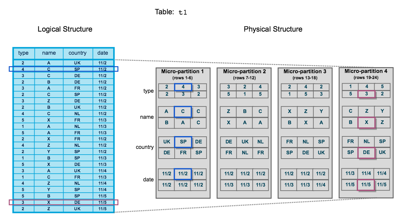
Each Snowflake table is divided into contiguous micro-partitions. Data within each micro-partition is stored in columnar format, compressed independently, and catalogued with rich metadata in the Cloud Services layer. Queries skip entire micro-partitions when the predicate values fall outside the stored min/max range for a column.
Key Characteristics of Micro-Partitions
| Property | Value |
|---|---|
| Size (compressed) | 50 MB – 500 MB |
| Storage format | Columnar (PAX-style) |
| Creation | Automatic — no manual definition |
| Immutability | Immutable once written |
| Compression | Automatic, per-column |
| Metadata | Stored in Cloud Services layer |
Once a micro-partition is written, it cannot be modified. Any DML operation (UPDATE, DELETE, MERGE) causes Snowflake to write entirely new micro-partitions and mark the old ones as deleted. This is why Snowflake’s Time Travel is possible — old micro-partitions are retained for the duration of the Time Travel period.
2. Micro-Partition Metadata
Snowflake automatically tracks rich metadata for every micro-partition, stored at the column level in the Cloud Services layer. This metadata is the engine that powers query pruning.
Per-Column Metadata in Every Micro-Partition
For each column in each micro-partition, Snowflake records four key statistics: minimum value, maximum value, number of distinct values (NDV), and null count. This metadata is stored in the Cloud Services layer, not inside the micro-partition data files themselves, so querying it costs no compute.

The Four Metadata Fields (Per Column, Per Micro-Partition)
- Min value — the smallest value present in that column within this micro-partition
- Max value — the largest value present in that column within this micro-partition
- NDV (Number of Distinct Values) — the cardinality of the column within this micro-partition
- Null count — how many null values exist in the column within this micro-partition
Because micro-partition metadata lives in the Cloud Services layer, Snowflake can evaluate whether to skip a micro-partition entirely before ever reading from cloud object storage. This means pruning decisions happen with zero virtual warehouse compute cost.
3. Query Pruning (Partition Elimination)
Query pruning is Snowflake’s mechanism for skipping micro-partitions that cannot possibly contain rows matching a query’s WHERE clause. This dramatically reduces I/O and accelerates analytical queries.
How Pruning Works
When you run a query with a filter predicate, Snowflake’s Cloud Services layer:
- Reads the metadata (min/max) for the filtered column across all micro-partitions
- Compares the predicate value to each micro-partition’s min/max range
- Marks any micro-partition where the predicate value falls outside the min/max range as pruned
- Sends only the surviving micro-partitions to the virtual warehouse for scanning
1-- Assume the ORDERS table has 10,000 micro-partitions2-- and ORDER_DATE is stored in insertion order (chronological)3SELECT4 order_id,5 customer_id,6 total_amount7FROM orders8WHERE order_date BETWEEN '2024-01-01' AND '2024-03-31';910-- Snowflake reads ORDER_DATE min/max for all 10,000 micro-partitions11-- Micro-partitions where max(order_date) < '2024-01-01' → PRUNED12-- Micro-partitions where min(order_date) > '2024-03-31' → PRUNED13-- Only micro-partitions that OVERLAP the range are scanned14-- Check pruning efficiency in Query Profile → "Partitions scanned" vs "Partitions total"After running a query, open the Query Profile in Snowsight. Under the TableScan operator you will see two metrics:
- Partitions total — all micro-partitions in the table
- Partitions scanned — micro-partitions that were actually read
A large difference between these two numbers indicates effective pruning. If partitions scanned ≈ partitions total, your data may benefit from a clustering key.
4. Natural Clustering
Before you define any explicit clustering key, Snowflake naturally orders data within micro-partitions based on insertion order. This is called natural clustering.
Natural Clustering via Insertion Order
When rows are inserted chronologically (e.g., daily ETL loads appending new records), each new micro-partition naturally contains data from a specific time period. A query filtering on a recent date range will automatically prune older micro-partitions without any clustering key defined.
When Natural Clustering is Sufficient
- Time-series tables loaded chronologically (e.g., event logs, transaction history)
- Append-only tables where new data always represents newer time periods
- Small-to-medium tables where full scans are fast regardless
As tables grow and accumulate updates, deletes, and out-of-order inserts, natural clustering degrades. Micro-partitions that once contained data from a single time period become mixed. This is when you should evaluate whether a clustering key and Automatic Clustering are warranted.
5. Clustering Keys
A clustering key is one or more columns (or expressions) that you designate as the primary sort dimension for a table. When a clustering key is defined, Snowflake will re-sort data into new micro-partitions optimised for pruning on those columns.
Defining a Clustering Key
1-- Option 1: Define clustering key at table creation2CREATE TABLE sales (3 sale_id NUMBER,4 sale_date DATE,5 region VARCHAR(50),6 product_id NUMBER,7 amount NUMBER(12,2)8)9CLUSTER BY (sale_date, region);1011-- Option 2: Add clustering key to an existing table12ALTER TABLE sales CLUSTER BY (sale_date, region);1314-- Option 3: Use an expression as a clustering key15-- Useful when you want to cluster on a derived value16ALTER TABLE events CLUSTER BY (DATE_TRUNC('month', event_timestamp));1718-- Remove a clustering key entirely19ALTER TABLE sales DROP CLUSTERING KEY;2021-- Suspend Automatic Clustering (keeps key definition, pauses background re-clustering)22ALTER TABLE sales SUSPEND RECLUSTER;2324-- Resume Automatic Clustering25ALTER TABLE sales RESUME RECLUSTER;When defining a composite clustering key with multiple columns, the order of columns matters. Snowflake clusters primarily by the first column, then by the second within each first-column bucket, and so on. Place the column with the highest cardinality and most selective queries first. Example: CLUSTER BY (region, sale_date) is optimal if queries almost always filter on region first.
When to Use Clustering Keys
Should You Define a Clustering Key?
6. Measuring Cluster Quality: Cluster Depth
Snowflake provides the SYSTEM$CLUSTERING_INFORMATION function to evaluate how well-clustered a table is on a given set of columns.
1-- Check clustering information for a table on a specific column set2SELECT SYSTEM$CLUSTERING_INFORMATION('sales', '(sale_date, region)');34-- Example output (JSON):5-- {6-- "cluster_by_keys" : "LINEAR(SALE_DATE, REGION)",7-- "total_partition_count" : 1250,8-- "total_constant_partition_count" : 42,9-- "average_overlaps" : 3.14,10-- "average_depth" : 2.87, ← Lower is better. 1.0 = perfectly clustered11-- "partition_depth_histogram" : {12-- "00000" : 42,13-- "00001" : 418,14-- "00002" : 561,15-- "00003" : 22916-- }17-- }1819-- Key metrics to interpret:20-- average_depth: ideally < 3. Higher means poor clustering (more overlap between micro-partitions)21-- average_overlaps: how many other micro-partitions share overlapping key ranges22-- total_constant_partition_count: micro-partitions with only one distinct key value (perfectly prunable)2324-- Check the AUTOMATIC_CLUSTERING_HISTORY view to see re-clustering activity25SELECT *26FROM SNOWFLAKE.ACCOUNT_USAGE.AUTOMATIC_CLUSTERING_HISTORY27WHERE TABLE_NAME = 'SALES'28ORDER BY START_TIME DESC29LIMIT 10;The exam tests whether you can interpret cluster depth values. Remember: lower cluster depth = better clustering. A depth of 1 means each micro-partition’s key range is unique with no overlap — perfect pruning. A depth of 10 means a query filtering on a specific value must scan an average of 10 micro-partitions for every logical key value.
7. Automatic Clustering
Automatic Clustering is a Snowflake-managed serverless service that continuously monitors a clustered table and triggers background re-clustering when the cluster depth degrades beyond a threshold.
Setting Up Automatic Clustering on a Large Table
Evaluate whether clustering is needed
Run a representative query and check Query Profile. Compare 'Partitions scanned' to 'Partitions total'. Also run SYSTEM$CLUSTERING_INFORMATION to get a baseline cluster depth.
SELECT SYSTEM$CLUSTERING_INFORMATION('my_large_table', '(event_date, region)');Define the clustering key on the table
Use ALTER TABLE ... CLUSTER BY to add the clustering key. Choose columns that appear most frequently in WHERE clauses. This action alone enables Automatic Clustering.
ALTER TABLE my_large_table CLUSTER BY (event_date, region);Monitor re-clustering progress
Query AUTOMATIC_CLUSTERING_HISTORY in SNOWFLAKE.ACCOUNT_USAGE to see when re-clustering jobs ran, how many credits were consumed, and how many bytes were processed.
SELECT
  table_name,
  start_time,
  end_time,
  credits_used,
  bytes_reclustered,
  partitions_reclustered
FROM SNOWFLAKE.ACCOUNT_USAGE.AUTOMATIC_CLUSTERING_HISTORY
WHERE table_name = 'MY_LARGE_TABLE'
ORDER BY start_time DESC;Validate improvement with SYSTEM$CLUSTERING_INFORMATION
After re-clustering completes, re-run the clustering information function. You should see average_depth decrease. Re-run your representative query and compare Partitions scanned.
SELECT SYSTEM$CLUSTERING_INFORMATION('my_large_table', '(event_date, region)');Optionally suspend clustering on non-production tables
If the table enters a read-only phase (e.g., archival), you can suspend Automatic Clustering to stop incurring serverless credits while preserving the clustering key definition.
ALTER TABLE my_large_table SUSPEND RECLUSTER;Automatic Clustering consumes serverless credits — not your warehouse credits. Costs depend on the amount of data re-clustered. Enabling clustering on a table with frequent random inserts and updates can generate significant ongoing costs. Always evaluate the query performance improvement vs. the re-clustering cost before enabling.
8. Table Types and Storage Costs
Snowflake has three table types with different storage cost profiles. Understanding the differences is critical for both the exam and real-world cost optimisation.
Snowflake Table Types: Storage Cost Comparison
Temporary tables behave like transient tables (no fail-safe, up to 1-day Time Travel) but are additionally scoped to the session — they are automatically dropped when the session ends. They are ideal for intermediate query results within a single session and are not visible to other sessions.
1-- Transient table: persists across sessions, no fail-safe2CREATE TRANSIENT TABLE staging.order_staging (3 order_id NUMBER,4 raw_json VARIANT,5 loaded_at TIMESTAMP_NTZ DEFAULT CURRENT_TIMESTAMP()6)7DATA_RETENTION_TIME_IN_DAYS = 1; -- max for transient89-- Temporary table: session-scoped, dropped automatically when session ends10CREATE TEMPORARY TABLE session_work.calc_results (11 customer_id NUMBER,12 lifetime_value NUMBER(12,2)13);1415-- Convert a permanent table to transient (must recreate)16-- There is no ALTER TABLE ... SET TYPE = TRANSIENT in Snowflake17-- You must CREATE TRANSIENT TABLE ... AS SELECT * FROM original_table1819-- Check current table type20SHOW TABLES LIKE 'ORDER_STAGING' IN SCHEMA staging;21-- Look at the "kind" column: TABLE (permanent), TRANSIENT, TEMPORARY9. Storage Metrics: TABLE_STORAGE_METRICS
Snowflake provides the INFORMATION_SCHEMA.TABLE_STORAGE_METRICS view (and the SNOWFLAKE.ACCOUNT_USAGE.TABLE_STORAGE_METRICS view for historical data) to inspect exactly how much storage each table is consuming across its three storage layers.
1-- Per-table storage breakdown (current state)2SELECT3 table_schema,4 table_name,5 table_type,6 -- Active data currently in the table7 ROUND(active_bytes / POWER(1024, 3), 2) AS active_gb,8 -- Data retained for Time Travel (deleted/updated rows still accessible via AT/BEFORE)9 ROUND(time_travel_bytes / POWER(1024, 3), 2) AS time_travel_gb,10 -- Data retained in fail-safe (7 days for permanent, 0 for transient/temporary)11 ROUND(failsafe_bytes / POWER(1024, 3), 2) AS failsafe_gb,12 -- Total billed storage13 ROUND((active_bytes + time_travel_bytes + failsafe_bytes) / POWER(1024, 3), 2) AS total_billed_gb14FROM information_schema.table_storage_metrics15WHERE active_bytes > 016ORDER BY total_billed_gb DESC;1718-- Find tables with the most fail-safe storage (potential cost saving opportunity)19SELECT20 table_name,21 ROUND(failsafe_bytes / POWER(1024, 3), 2) AS failsafe_gb22FROM information_schema.table_storage_metrics23WHERE failsafe_bytes > 1073741824 -- > 1 GB in fail-safe24ORDER BY failsafe_bytes DESC;2526-- Identify staging tables that should probably be TRANSIENT27SELECT28 table_name,29 table_type,30 ROUND(failsafe_bytes / POWER(1024, 3), 2) AS failsafe_gb31FROM information_schema.table_storage_metrics32WHERE table_name ILIKE '%staging%'33AND table_type = 'BASE TABLE' -- permanent, not transient34ORDER BY failsafe_bytes DESC;The exam frequently tests understanding of Snowflake’s three storage billing components. Remember: active_bytes + time_travel_bytes + failsafe_bytes = total billed. Transient tables have no failsafe_bytes. Temporary tables have neither failsafe_bytes nor cross-session persistence. Using transient tables for staging data is a common cost-optimisation strategy tested in scenario questions.
10. Columnar vs Row-Based Storage
Snowflake stores data in a columnar format. This is one of the most important architectural decisions underpinning its analytical performance. Understanding why columnar beats row-based storage for OLAP workloads is tested in the COF-C02 exam.
Columnar vs Row-Based Storage Layout
In row-based storage (left), all columns for a single row are stored contiguously. To read a single column across millions of rows, the database must scan every byte of every row. In columnar storage (right), all values for a single column are stored contiguously. Reading one column across millions of rows requires only a tiny fraction of the total I/O, and values within a column compress far more efficiently because they share the same data type and often similar values.
Columnar vs Row-Based Storage for Analytics
Key Terms
Data Storage & Clustering Key Terms
Micro-partition
The fundamental unit of Snowflake storage. Each micro-partition is a contiguous slice of a table, stored in columnar format, automatically sized between 50–500 MB compressed, and immutable once written.
Query pruning
The process by which Snowflake's Cloud Services layer compares query predicate values to per-column min/max metadata and skips micro-partitions that cannot contain matching rows, reducing I/O.
Clustering key
One or more columns (or expressions) designated as the primary sort dimension for a table. Enables Snowflake to re-organise data into micro-partitions that are optimally prunable for queries filtering on those columns.
Cluster depth
A metric returned by SYSTEM$CLUSTERING_INFORMATION indicating the average number of micro-partitions that contain overlapping key ranges. Lower values indicate better clustering. Ideal value is close to 1.
Automatic Clustering
A Snowflake-managed serverless service that continuously monitors a clustered table's depth and triggers background re-clustering jobs when degradation is detected. Charged as serverless credits.
Number of Distinct Values
A per-column metadata statistic stored for each micro-partition indicating the cardinality (count of unique values) within that micro-partition. Part of the four key metadata fields tracked.
Fail-safe
A 7-day period following the Time Travel retention window during which Snowflake retains deleted or expired micro-partition data. Data can only be recovered by Snowflake Support. Only applies to permanent tables.
Transient table
A Snowflake table type with no fail-safe period and a maximum of 1 day of Time Travel retention. Lower storage cost than permanent tables. Suitable for staging and ETL intermediate data.
Natural clustering
The implicit ordering of data within micro-partitions based on insertion order, without any defined clustering key. Works well for chronologically loaded time-series data.
TABLE_STORAGE_METRICS
An INFORMATION_SCHEMA view that reports active_bytes, time_travel_bytes, and failsafe_bytes per table, enabling detailed analysis of storage costs across Snowflake table types.
Flashcard Review
What is the compressed size range of a Snowflake micro-partition?
50 MB to 500 MB compressed. Snowflake automatically determines the exact size — you cannot configure it. Micro-partitions are contiguous, immutable, and stored in columnar format.
What four metadata statistics does Snowflake store per column per micro-partition?
1. Min value — smallest value in that column within the micro-partition. 2. Max value — largest value. 3. NDV (Number of Distinct Values) — cardinality within the micro-partition. 4. Null count — number of null values. This metadata is stored in the Cloud Services layer and used for query pruning.
What does a cluster depth of 1.0 indicate versus a depth of 8.0?
A cluster depth of 1.0 means each micro-partition has a unique, non-overlapping key range — perfect clustering. A depth of 8.0 means an average of 8 micro-partitions share overlapping key ranges for any given key value — poor clustering requiring more micro-partitions to be scanned per query.
What are the three storage cost components billed by Snowflake for a permanent table?
1. Active bytes — current live data. 2. Time Travel bytes — data retained within the Time Travel retention window (0–90 days for permanent tables). 3. Fail-safe bytes — data retained for 7 days after Time Travel expires. Transient tables have no fail-safe bytes. Visible via INFORMATION_SCHEMA.TABLE_STORAGE_METRICS.
Name two situations where you should NOT define a clustering key on a Snowflake table.
1. Small tables (< 1 TB) — full micro-partition scans are fast enough that the overhead and cost of Automatic Clustering is not justified. 2. Highly volatile tables with frequent updates/deletes — constant DML triggers constant re-clustering, generating significant and continuous serverless credit consumption.
Practice Quizzes
A data engineer notices that a query scanning a 5 TB SALES table reads 98% of all micro-partitions every time. The WHERE clause filters on SALE_DATE. What is the MOST likely cause?
Which Snowflake function returns the average cluster depth of a table for a given set of columns?
An organisation has a STAGING_ORDERS table used only as an ETL landing zone. Data is loaded, transformed, and moved to production tables within 24 hours. The table currently accumulates significant fail-safe storage costs. What table type change would ELIMINATE fail-safe costs?
Cheat Sheet
Data Storage & Clustering — COF-C02 Quick Reference
Micro-Partition Facts
SizeFormatMutabilityMetadata locationMetadata fieldsClustering Commands
Add clustering keyRemove clustering keySuspend re-clusteringCheck cluster depthView AC historyTable Type Storage
PermanentTransientTemporaryStorage viewWhen to Cluster
DO clusterDO NOT clusterCluster cost typeIdeal cluster depthSummary
Snowflake’s storage architecture is built on immutable, columnar micro-partitions that are automatically sized and created without any DBA intervention. The rich per-column metadata stored in the Cloud Services layer powers query pruning — the ability to skip entire micro-partitions without reading them — which is fundamental to Snowflake’s query performance.
Natural clustering works well for chronologically loaded time-series data, but large tables with varied query patterns benefit from explicitly defined clustering keys. Automatic Clustering maintains cluster quality continuously as a serverless background service, charged separately from virtual warehouse credits.
For the COF-C02 exam, internalise:
- Micro-partition size: 50–500 MB compressed
- Metadata tracked: min, max, NDV, null count per column per micro-partition
- Cluster depth: lower is better, check with
SYSTEM$CLUSTERING_INFORMATION - Clustering cost: serverless credits (not warehouse credits)
- Table types: permanent (fail-safe 7d) vs transient (no fail-safe) vs temporary (session-scoped, no fail-safe)
- Storage billing: active + time_travel + failsafe bytes, visible in
INFORMATION_SCHEMA.TABLE_STORAGE_METRICS
Reinforce what you just read
Study the All flashcards with spaced repetition to lock it in.